42 conditional formatting pivot table row labels
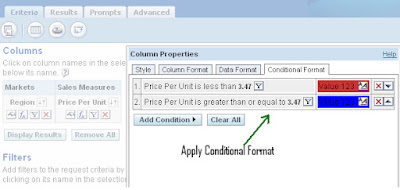
exceljet.net › pivot-table-tipsPivot Table Tips - Exceljet Drag a "label" field into the Row Labels area (e.g. customer) Drag a numeric field into the Values area (e.g. sales) A basic pivot table in about 30 seconds. The pivot table above shows total sales by product, but you can can easily rearrange fields to show total sales by region, by category, by month, and so on. How to Apply Conditional Formatting to Rows Based on Cell Value On the Home tab of the Ribbon, select the Conditional Formatting drop-down and click on Manage Rules…. That will bring up the Conditional Formatting Rules Manager window. Click on New Rule. This will open the New Formatting Rule window. Under Select a Rule Type, choose Use a formula to determine which cells to format.
Conditional Formatting in Pivot Table - WallStreetMojo We must follow the steps to apply conditional formatting in the pivot table. First, we must select the data. Then, in the "Insert" Tab, click on "Pivot Tables." As a result, a dialog box appears. Next, we must insert the pivot table in a new worksheet by clicking "OK." Currently, a pivot table is blank. Next, we need to bring in the values.
Conditional formatting pivot table row labels
How to apply conditional formatting to Pivot Tables Go to HOME > Conditional Formatting > New Rule to add a new formatting rule, or select from predefined options. If you select the latter, you will need to configure the rule regardless. The New (or Edit) Formatting Rule window contains options specific to Pivot Tables. You can choose the location where you want to apply your conditional ... trumpexcel.com › group-dates-in-pivot-tables-excelHow to Group Dates in Pivot Tables in Excel (by Years, Months ... Create a pivot table with Date in the Rows area and Resolved in the Values area. Select any cell in the Date column in the Pivot Table. Go to Pivot Table Tools –> Analyze –> Group –> Group Selection. In the Grouping dialogue box, select Hours. Click OK. This will group the data by hours and you will get something as shown below: Pivot Table Grouping, Ungrouping And Conditional Formatting #1) Select the entire column under the Sum of Total column in the pivot table. #2) Navigate to Home -> Conditional Formatting #3) Select Top/Bottom Rules -> Bottom 10 items. #4) In the dialog reduce the count to 3 (since we want just the bottom 3) and you can choose any highlighter from the drop-down.
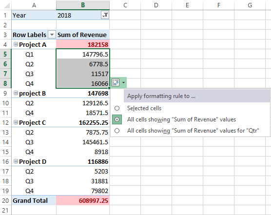
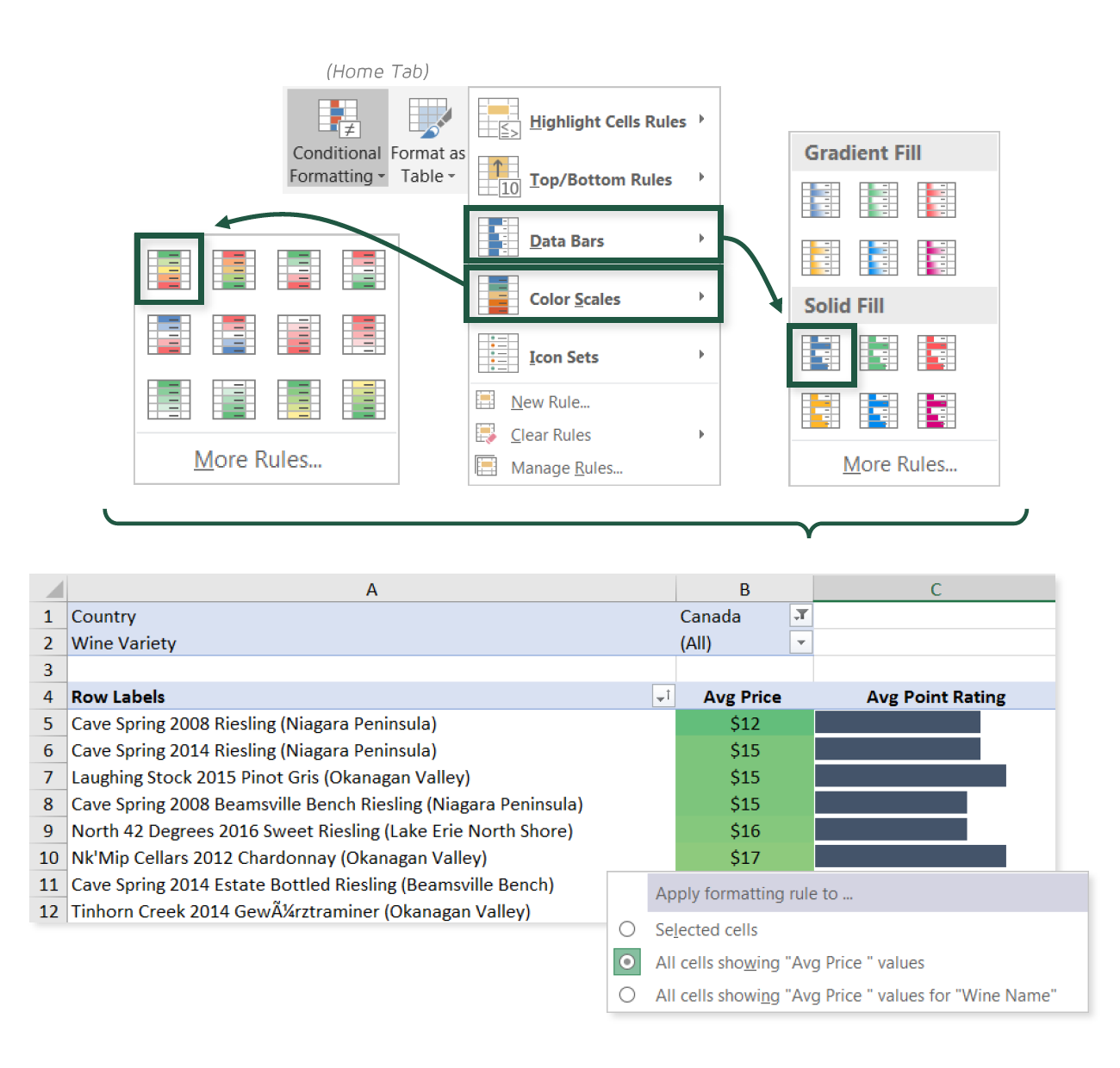
Conditional formatting pivot table row labels. Apply Conditional Formatting | Excel Pivot Table Tutorial First of all, select any of the cells which have month value. Then, go to Home Tab → Styles → Conditional Formatting → New Rule. Here, you will get a pop-up window to apply conditional formatting to the pivot table. In this pop-up window, you have three different options to apply conditional formatting in pivot table. conditional formatting per row on pivot - Microsoft Tech Community conditional formatting per row on pivot. I would like to format each row of a pivot table separately (as in the picture shown below), but I cannot paste the formatting. I've got many rows, and they could change (just like the columns) Is there a way to automate this, or I have to select row by row and apply the formatting? Conditional Formatting in Pivot Table (Example) - EDUCBA Click on any cell in the pivot table > Go to the HOME tab > Click on Conditional Formatting option under Styles option > Click on Manage Rules option. It will open a Rules Manager dialog box. Click on the Edit Rule tab, as shown in the below screenshot. It will open the Editing Rule formatting window. Refer to the below screenshot. › Conditional-formatting-ExcelConditional Formatting in Excel - a Beginner's Guide Here’s what the pivot table looks like when it’s condensed to the top 15 countries. Notice in the image above, the Row Labels and Column Labels header drop downs are missing. For a cleaner look to your pivot table, you can hide your row label and column labels. On the Pivot Table Analyze tab, just click Field Headers to make them disappear ...
Conditional Formatting on Pivot Table row labels In srcFromPowerPivot sheet cell A is from powerpivot under row label comparing the dates in cell C (3 dates) and the condtional formatting doesnt work. In cell J it worked cos I dragged under value instead of row label. In the srcFromWorksheet it worked even though it is under rowlabel. Sheet3 is just a copy of powerpivot data. Issue with conditional formatting in pivot table | General Excel ... I made a pivot table to present three years data and highlighted the numbers > 249 with conditional formatting in the pivot table. ... i.e. not PivotTable conditional formatting. Apply it to the column, where the row label contains 'Total'. If you get stuck, please start a new thread as it will be off topic. Mynda. Forum Timezone: Australia ... Conditional formatting rows in a pivot table based on one rows criteria ... I am havong difficulty trying to highlight an entire row in a pivot table based on one rows criteria. The pivot table is from A:M and I need to highlight the corresponding row if column I has 992 in it. I have tried sevral ways but can only get it to work if I just focus on one row. I am at a loss for what I am doing wrong. Conditional Format Pivot Table Row - Chandoo.org Select the entire row, and when you apply the conditional format, make the column reference absolute. So, say we want the entire row 2 to be formatted if cell in col B = 5. formula would be: =$B2=5
Pivot Table Conditional Formatting for Different Rows Items? Hello, It is possible! All you have to do: Select Your Pivot Table and: Go to Conditional Formatting -> New Rule -> Choose All cells showing "duration" values for "Type and "Date Selection" under "Apply Rule To" section -> Use a Formula to Determine which cells to format and enter the following formula: =AND(A6="Cars",A6>3), You can create new rules for other two conditions as well: Excel VBA: Conditional Format of Pivot Table based on Column Label myPivotSourceName = myPivotField.Name. Then rather than referencing the data field with the pivot field object, I referenced the DataRange with the string: myPivotTable.PivotFields (myPivotSourceName).DataRange.Select. Works perfectly and is completely portable for any pivottable on any sheet with any fields. excel vba. › pivot-tables › pivot-tableHow to Apply Conditional Formatting to Pivot Tables Dec 13, 2018 · Great question! I don’t believe there is a direct way to do this with the conditional formatting setting for the pivot table. Those settings are applied at the pivot field level, and not the pivot item level. In the example of Quarters, each quarter (Q1, Q2, Q3, Q4) would be a pivot item. The conditional formatting is applied at the field level. › pivottabletextvaluesHow to Show Text in Pivot Table Values Area Jan 27, 2022 · On the Excel Ribbon's Home tab, click Conditional Formatting; Then click New Rule, to open the New Formatting Rule dialog box; In the Apply Rule to section, select the 3rd option - All cells showing 'Max of RegID' values for 'City' and 'Store'. This option creates flexible conditional formatting that will adjust if the pivot table layout changes.
How to use conditional formatting in decorating pivot tables | Basic Excel Tutorial
How to make row labels on same line in pivot table? Make row labels on same line with PivotTable Options You can also go to the PivotTable Options dialog box to set an option to finish this operation. 1. Click any one cell in the pivot table, and right click to choose PivotTable Options, see screenshot: 2.

Pivot Table Row Labels In the Same Line - Beat Excel!
Format Pivot Table Labels Based on Date Range In the pivot table, remove any filters that have been applied - all the rows need to be visible before you apply the conditional formatting. Select all the dates in the Row Labels that you want to format. On the Ribbon, click the Home tab, and then in the Styles group, click Conditional Formatting.
ORACLE BUSINESS INTELLIGENCE ENTERPRISE EDITION 100: Conditional Formatting in Grand Total in ...
Conditional formatting for Pivot Tables in Excel 2016 - 2007 Conditional formatting when applied to PivotTables in Excel 2007 - 2016 is applied to the underlying structure of the PivotTable rather than to the cells themselves. So, when you interact with a PivotTable such as moving fields around and viewing your data in different ways, the formatting is updated as you work.
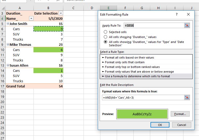
Pivot Table Conditional Formatting for Different Rows Items? - Microsoft Community
Overwrite pivot table conditional format based on row label As far as I know, using the one rule in the Conditional formatting, we can only format the cells with one color if the condition is true and if the same condition is false, the formatting of the cell will be blank and if both conditions are true, the formatting of cell depends on the highest ranking/priority of the rules in Conditional formatting.
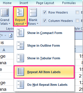
How to repeat row labels for group in pivot table?
Pivot Table Conditional Formatting with VBA - Peltier Tech sub formatpt1 () dim c as range with activesheet.pivottables ("pivottable1") ' reset default formatting with .tablerange1 .font.bold = false .interior.colorindex = 0 end with ' apply formatting to each row if condition is met for each c in .databodyrange.cells if c.value >= 7 then with .tablerange1.rows (c.row - .tablerange1.row + 1) …
Conditional Pivot Table Formats | Excel Maven
spreadsheeto.com › pivot-tablesHow to Create a Pivot Table in Excel: Pivot Tables Explained To apply a conditional formatting rule to the entire Pivot Table, use the 2nd or 3rd options in the button that appears after using conditional formatting. Number formats Some data displays in an inherent logical way (e.g. currency starting with $ or £) .
How to repeat row labels for group in pivot table?
Pivot Table Conditional Formatting - Microsoft Tech Community Hi all :) I have an issue conditionally formatting a Pivot Table. I have my row hierarchy set up as Region, Area, Store, Consultant. My rows are expanded out only to a Store Level. I need the Store Name to be highlighted red if the value in the first column is <1. I have applied conditional fo...

How to Create a MS Excel Pivot Table – An Introduction | SIMPLE TAX INDIA
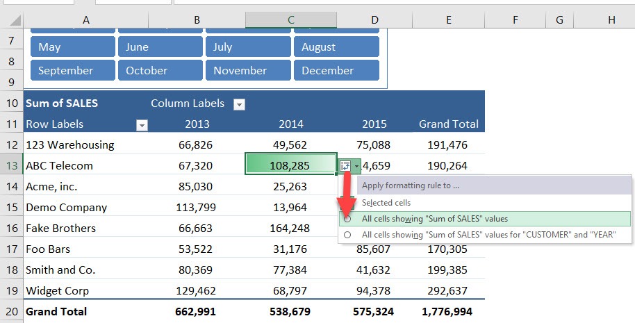
Pivot table conditional formatting - Exceljet Select any cell in the data you wish to format and then choose "New rule" from the conditional formatting menu on the Home tab of the ribbon. At the top of the window, you will see setting for which cells to apply conditional formatting to. For the example shown, we want: "All cells showing sum of "sales values" for name and "date"

How to use conditional formatting in decorating pivot tables | Basic Excel Tutorial
How to Format Excel Pivot Table - Contextures Excel Tips First, select a cell in the pivot table. Next, on the Excel Ribbon, click the Design tab. In the PivotTable Styles gallery, scroll to the bottom. Click the New PivotTable Style command. Next, follow the steps in the next section below, to name and modify the new style.

33 Pivot Table Blank Row Label - Labels Database 2020
Conditional Formatting PivotTables - My Online Training Hub Here's a step by step how to: 1. Select any cell in the values area of your PivotTable. 2. On the Home tab of the Ribbon select Conditional Formatting > Top/Bottom Rules > Top 10 Items: 3. Set the value to 1 and choose your format: 4. You will now have an icon beside the cell that you have applied the formatting to.

Accelerate Your Analysis with Pivot Table | Simplified Excel
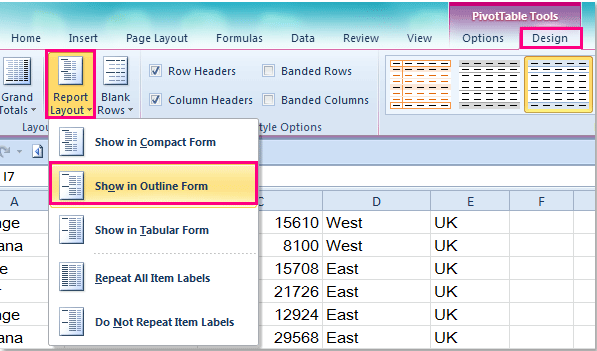
Design the layout and format of a PivotTable Right-click the field name and then select the appropriate command — Add to Report Filter, Add to Column Label, Add to Row Label, or Add to Values — to place the field in a specific area of the layout section. Click and hold a field name, and then drag the field between the field section and an area in the layout section.

How to Create a MS Excel Pivot Table – An Introduc
excelchamps.com › pivot-tablePivot Table Tutorial (100 Tips and Tricks) | Basic to Advanced Written by Puneet for Excel 2007, Excel 2010, Excel 2013, Excel 2016, Excel 2019, Excel for Mac. Pivot Tables are one of the Intermediate Excel Skills and this is an Advanced Pivot Table Tutorial that shows you the top 100 tips and tricks to master this skill.

March 2012 | OPTION EXPLICIT VBA
Add Pivot Table Conditional Formatting and Fix Problems To apply simple conditional formatting: In the pivot table, select the territory sales amounts, in cells B5:C16. On the Ribbon's Home tab, click Conditional Formatting. Click Top/Bottom Rules, and click Above Average. In the Above Average window, select one of the formatting options from the drop down list.

Conditional Formatting in Pivot Tables - YouTube
Excel Pivot Table Conditional Formatting Row Labels Go making the conditional formatting select the color scale and do it based on commercial and choose diverging and the colors should give expected result. Here a glaze color or bar and been applied...
Conditionally Format a Pivot Table With Data Bars | MyExcelOnline
How to preserve formatting after refreshing pivot table? In the PivotTable Options dialog box, click Layout & Format tab, and then check Preserve cell formatting on update item under the Format section, see screenshot: 4. And then click OK to close this dialog, and now, when you format your pivot table and refresh it, the formatting will not be disappeared any more.
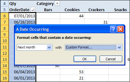
Format Pivot Table Labels Based on Date Range – Excel Pivot Tables
Pivot Table Grouping, Ungrouping And Conditional Formatting #1) Select the entire column under the Sum of Total column in the pivot table. #2) Navigate to Home -> Conditional Formatting #3) Select Top/Bottom Rules -> Bottom 10 items. #4) In the dialog reduce the count to 3 (since we want just the bottom 3) and you can choose any highlighter from the drop-down.
Post a Comment for "42 conditional formatting pivot table row labels"