45 excel chart vertical axis labels
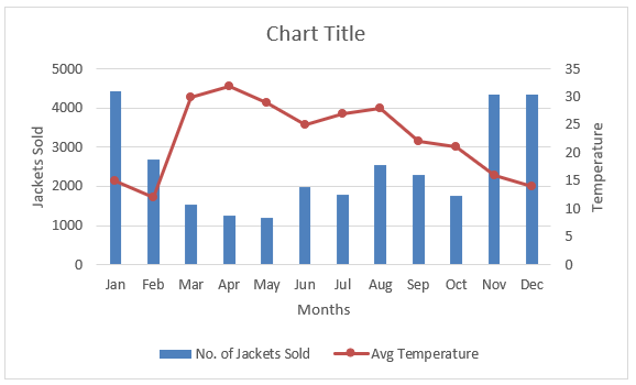
How to Create and Customize a Waterfall Chart in Microsoft Excel Select the chart and use the buttons on the right (Excel on Windows) to adjust Chart Elements like labels and the legend, or Chart Styles to pick a theme or color scheme. Select the chart and go to the Chart Design tab. How to make a 3 Axis Graph using Excel? - GeeksforGeeks To create a 3 axis graph follow the following steps: Step 1: Select table B3:E12.Then go to Insert Tab, and select the Scatter with Chart Lines and Marker Chart.. Step 2: A Line chart with a primary axis will be created. Step 3: The primary axis of the chart will be Temperature, the secondary axis will be Pressure and the third axis will be Volume.So, to create the third axis duplicate this ...
Axis.TickLabels property (Excel) | Microsoft Docs Returns a TickLabels object that represents the tick-mark labels for the specified axis. Read-only. Syntax. expression.TickLabels. expression A variable that represents an Axis object. Example. This example sets the color of the tick-mark label font for the value axis on Chart1. Charts("Chart1").Axes(xlValue).TickLabels.Font.ColorIndex = 3 ...

Excel chart vertical axis labels
Add Vertical Lines To Excel Charts Like A Pro! [Guide] Simply select your plotted dot and right-click on it. Then open the Add Data Labels menu and click Add Data Labels. You should then see a data label appear next to your vertical line. Next, you'll likely want to reposition your data label to be directly over your vertical line. Excel Chart Vertical Axis Text Labels • My Online Training Hub Hide the left hand vertical axis: right-click the axis (or double click if you have Excel 2010/13) > Format Axis > Axis Options: Set tick marks and axis labels to None; While you’re there set the Minimum to 0, the Maximum to 5, and the Major unit to 1. This is to suit the minimum/maximum values in your line chart. Custom Axis Labels and Gridlines in an Excel Chart 23/07/2013 · Select the vertical dummy series and add data labels, as follows. In Excel 2007-2010, go to the Chart Tools > Layout tab > Data Labels > More Data label Options. In Excel 2013, click the “+” icon to the top right of the chart, click the right arrow next to Data Labels, and choose More Options…. Then in all versions, choose the Label Contains option for Y Values …
Excel chart vertical axis labels. How to add a single vertical bar to a Microsoft Excel line chart The next step is to make the vertical bar extend beyond the $1,800,000 on the left by changing the secondary axis to its maximum boundary, which is 1,800,000. Doing so will extend the vertical bar.... › excel-chart-verticalExcel Chart Vertical Axis Text Labels - My Online Training Hub Hide the left hand vertical axis: right-click the axis (or double click if you have Excel 2010/13) > Format Axis > Axis Options: Set tick marks and axis labels to None; While you’re there set the Minimum to 0, the Maximum to 5, and the Major unit to 1. This is to suit the minimum/maximum values in your line chart. How to rotate axis labels in chart in Excel? - ExtendOffice Rotate axis labels in chart of Excel 2013. If you are using Microsoft Excel 2013, you can rotate the axis labels with following steps: 1. Go to the chart and right click its axis labels you will rotate, and select the Format Axis from the context menu. 2. In the Format Axis pane in the right, click the Size & Properties button, click the Text ... How to group (two-level) axis labels in a chart in Excel? The Pivot Chart tool is so powerful that it can help you to create a chart with one kind of labels grouped by another kind of labels in a two-lever axis easily in Excel. You can do as follows: 1. Create a Pivot Chart with selecting the source data, and: (1) In Excel 2007 and 2010, clicking the PivotTable > PivotChart in the Tables group on the ...
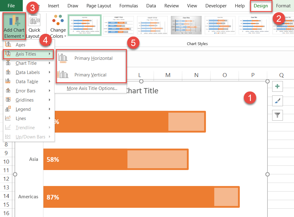
How to Change the Y Axis in Excel - Alphr Bring the cursor to the chart where you want to change the axes' appearance. Go to "Design," then go to "Add Chart Element" and "Axes." You'll have two options: "Primary Horizontal" will... Excel Charts with Shapes for Infographics - My Online Training Hub Start by inserting a regular column chart. Then insert the shape you want to use. Make sure it's roughly the same size as the largest column in your chart. CTRL+C to copy the Shape > Select the columns in the chart > CTRL+V to paste the shape. Tip: add data labels and remove the gridlines and vertical axis. Modifying Axis Scale Labels (Microsoft Excel) Create your chart as you normally would. Double-click the axis you want to scale. You should see the Format Axis dialog box. (If double-clicking doesn't work, right-click the axis and choose Format Axis from the resulting Context menu.) Make sure the Scale tab is displayed. (See Figure 2.) Figure 2. The Scale tab of the Format Axis dialog box. How to make a quadrant chart using Excel - Basic Excel Tutorial Right-click on any label and select 'Format Data Labels.' Go to the 'Label Options' tab and check the 'Value from cells' option. Select all the names and click OK. Uncheck the 'Y Value' box and under 'Label Position,' select 'Above. 7. Add the Axis titles. Select the chart and go to the 'Design' tab. Choose 'Add Chart Element' and click 'Axis ...
Add or remove a secondary axis in a chart in Excel To plot more than one data series on the secondary vertical axis, repeat this procedure for each data series that you want to display on the secondary vertical axis. In a chart, click the data series that you want to plot on a secondary vertical axis, or do the following to select the data series from a list of chart elements: Click the chart. Make Excel charts primary and secondary axis the same scale These series may be hard to see so the easiest way to customise them is to click on the Chart, click on the Format tab, and find the series called Primary Scale. Just below this dropdown you can click on Format Selection. On the resultant options box, change the fill to No Fill and the Border to No line. You will do the same for the other new ... 100% Stacked Area Chart in Excel - Excel Unlocked To insert a 100% Stacked Area Chart, follow the steps:-. Select the range A1:E6. Go to Insert tab. In the charts group, click on Recommended Charts button. The insert chart dialog box opens. Go to All Charts tab and Click on Area Charts from the menu. Select the 100% Stacked Area chart from there. Chart.Axes method (Excel) | Microsoft Docs This example adds an axis label to the category axis on Chart1. VB. With Charts ("Chart1").Axes (xlCategory) .HasTitle = True .AxisTitle.Text = "July Sales" End With. This example turns off major gridlines for the category axis on Chart1. VB.

IT Training Tips: Indiana University » Blog Archive » Combination Charts and Secondary Axes in Excel
How do I stop the data label's text direction rotating every time ... Victoria Makepeace. Replied on October 27, 2021. In reply to Minhokiller's post on October 27, 2021. I'm not sure to be honest, it started to do this when I click on Select Data and highlight the data sources. I do get 1 bar/data labels that's in the correct text direction (vertical) but all of the other bars/data labels are horizonal.

How to Add Axis Labels in Excel - BSUPERIOR
peltiertech.com › text-labels-on-horizontal-axis-in-eText Labels on a Horizontal Bar Chart in Excel - Peltier Tech Dec 21, 2010 · In Excel 2003 the chart has a Ratings labels at the top of the chart, because it has secondary horizontal axis. Excel 2007 has no Ratings labels or secondary horizontal axis, so we have to add the axis by hand. On the Excel 2007 Chart Tools > Layout tab, click Axes, then Secondary Horizontal Axis, then Show Left to Right Axis.

How to add axis label to chart in Excel?
› documents › excelHow to group (two-level) axis labels in a chart in Excel? The Pivot Chart tool is so powerful that it can help you to create a chart with one kind of labels grouped by another kind of labels in a two-lever axis easily in Excel. You can do as follows: 1. Create a Pivot Chart with selecting the source data, and: (1) In Excel 2007 and 2010, clicking the PivotTable > PivotChart in the Tables group on the ...
Combination Charts in Excel (Examples) | Steps to Create Combo Chart
Two-Level Axis Labels (Microsoft Excel) - ExcelTips (ribbon) Excel automatically recognizes that you have two rows being used for the X-axis labels, and formats the chart correctly. Since the X-axis labels appear beneath the chart data, the order of the label rows is reversed—exactly as mentioned at the first of this tip. (See Figure 1.) Figure 1. Two-level axis labels are created automatically by Excel.

Moving X-axis labels at the bottom of the chart below negative values in Excel - PakAccountants.com
Excel Chart Axis Switch • My Online Training Hub The switch buttons are linked to cell W18 in the worksheet. Excel detects which button is selected (button 1 or button 2) and enters the number in the cell. I can then reference this cell in formulas to choose which axis to display. The axis to display is handled by a ghost series which is an additional hidden series in each chart that plots ...
Excel chart with a single x-axis but two different ranges (combining horizontal clustered bar ...
How to make shading on Excel chart and move x axis labels to the bottom ... For the yellow shading, add a series with constant value -80, and a series with constant value -20. In the Change Chart Type dialog, change the chart type for the new series to Stacked Area. Change the color from whatever Excel decides to yellow. Finally, remove the new series form the legend. See the attached version. Wi-Fi Signal Strength.xlsx
How to Create Progress Charts (Bar and Circle) in Excel - Automate Excel
Horizontal axis labels on a chart - Microsoft Community If you start with Jan or January, then fill down, Excel should automatically fill in the following names. Click on the chart. Click 'Select Data' on the 'Chart Design' tab of the ribbon. Click Edit under 'Horizontal (Category) Axis Labels'. Point to the range with the months, then OK your way out. --- Kind regards, HansV
Create a Custom Number Format for a Chart Axis - YouTube
Text Labels on a Horizontal Bar Chart in Excel - Peltier Tech 21/12/2010 · In Excel 2003 the chart has a Ratings labels at the top of the chart, because it has secondary horizontal axis. Excel 2007 has no Ratings labels or secondary horizontal axis, so we have to add the axis by hand. On the Excel 2007 Chart Tools > Layout tab, click Axes, then Secondary Horizontal Axis, then Show Left to Right Axis.
Post a Comment for "45 excel chart vertical axis labels"